Introduction

Since its introduction in 2017, the Transformer has become the foundation of modern deep learning, powering large language models, vision transformers, and many multimodal architectures. Although libraries such as PyTorch and Hugging Face provide highly optimized implementations, they often abstract away the mathematical ideas that make the architecture work.

In this article, we will reimplement the original Transformer proposed in Attention Is All You Need from scratch using PyTorch. Rather than relying on high-level modules like nn.Transformer, we will build every component ourselves, translating the equations from the paper into clean, modular code.

Our goal is not to reproduce the latest Transformer variants or incorporate modern improvements such as Rotary Position Embeddings (RoPE), FlashAttention, or SwiGLU. Instead, we will faithfully follow the original 2017 architecture, implementing each building block exactly as described by the authors.

Throughout the article, we will:

• derive the mathematical formulation of each component,
• develop the intuition behind its design,
• implement it from scratch in PyTorch, and
• verify that the implementation behaves as expected before assembling the complete model.

By the end, we will have reconstructed the entire Transformer—from token embeddings and positional encodings to multi-head attention, encoder and decoder layers, and the final sequence-to-sequence architecture—providing a clear bridge between the original paper and a working implementation.

1. Token Embeddings

Background

The first component of the Transformer architecture is the token embedding layer. Neural Networks operate better on continuous vectors compared to discrete token IDs, so the first step would be to map every token to a learned dense representation.

Now, given a input sequence,

each token is looked up in a learnable embedding matrix $E \in \mathbb{R}^{ |V| \times d_{model}}$, where $|V|$ is the size of the vocabulary and $d_{model}$ is the dimension of the embedding vectors.

Each row in $E$ represents the embedding corresponding to a token in the vocabulary. Therefore for a token $x_i$, its corresponding embedding

which is basically the $x_i^{th}$ row in the embedding matrix.

Scaling

However, there is all small detail mentioned in the paper which we need to account for.

In the embedding layers, we multiply those weights by $\sqrt{d_{model}}$

Thus the output of the embedding layer is

where $z_i \in \mathbb{R}^{d_{model}}$

This is due to the fact that immediately after the token embedding we need to add positional embeddings. Scaling the embeddings helps keep their magnitude comparable to that of the positional embeddings, preventing either component from dominating the combined representation during the forward pass.

PyTorch Implementation

class TokenEmbedding(nn.Module):
    def __init__(self, vocab_size:int, d_model: int):
        super().__init__()
 
        self.d_model = d_model
        self.embedding = nn.Embedding(vocab_size, d_model)
 
    def forward(self, x):
        """
        Args:
            x: (batch, seq_len)
        Returns:
            (batch, seq_len, d_model)
        """
        return self.embedding(x) * math.sqrt(self.d_model)
 

2. Positional Encodings

Background

Since our model contains no recurrence and no convolution, in order for the model to make use of the order of the sequence, we must inject some information about the relative or absolute position of the tokens in the sequence. To this end, we add "positional encodings" to the input embeddings ...

As the authors have mentioned in the paper, we need to add the sense of positions in the architecture since further calculations are permutation invariant in nature. In other words, the order of the tokens i.e. swapping the position of any two tokens does not change the output of the model. So we add positional encodings to the input embeddings to give the model a sense of position.

Formulae

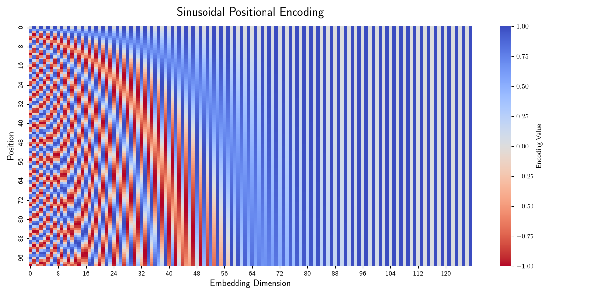
The authors decided to use sine and cosine functions to generate sinusoidal positional encodings. The idea is to use different frequencies of sine and cosine functions to generate different positional encodings.

where $pos$ is the position of the token in the sequence and $i$ is the dimension of the embedding vector.

PyTorch Implementation

class SinusoidalPositionalEncoding(nn.Module):
    def __init__(self, d_model: int, max_len:int=5000, dropout=0.1):
        super().__init__()
 
        pe = torch.zeros(max_len, d_model)
        positions = torch.arange(max_len).unsqueeze(1)
 
        div_term = torch.exp(torch.arange(0, d_model, 2)* (-math.log(10000.0) / d_model))
        
        pe[:, 0::2] = torch.sin(positions * div_term)
        pe[:, 1::2] = torch.cos(positions * div_term)
 
        pe = pe.unsqueeze(0)
 
        self.dropout = nn.Dropout(dropout)
        self.register_buffer("pe", pe)
    
    def forward(self, x: torch.Tensor) -> torch.Tensor:
        """
        Adds positional encodings to the input embeddings and applies dropout.
 
        Args:
            x: Input tensor of shape (batch_size, seq_len, d_model).
 
        Returns:
            Tensor of the same shape with positional encodings added and dropout applied.
        """
        x = x + self.pe[:, :x.size(1)]
        return self.dropout(x)

Visualization

import matplotlib.pyplot as plt
import seaborn as sns
 
d_model, max_len = 128, 100
spe = SinusoidalPositionalEncoding(d_model, max_len)
 
def plot_spe(spe):
    plt.figure(figsize=(12, 6))
    sns.heatmap(spe.pe.squeeze(0),cmap="coolwarm_r",
        xticklabels=8,yticklabels=8,
        cbar_kws={"label": "Encoding Value"},
    )
    plt.title("Sinusoidal Positional Encoding", fontsize=18, weight="bold", pad=15)
    plt.xlabel("Embedding Dimension", fontsize=13)
    plt.ylabel("Position", fontsize=13)
    plt.tight_layout()
    plt.show()
    
plot_spe(spe)